Support Vector Machine

SVM(Support Vector Machine) is a machine learning algorithm used for both classification and regression problem.It is mainly used for Classification problem in which the set of training examples is divided into further parts. we perform classification by finding the hyper-plane that differentiate the two classes very well (look at the below snapshot).

There are ways by which we can plot a SVM:-

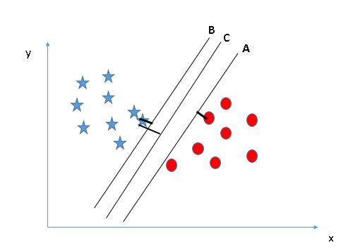
Identify the right hyper-plane (Scenario-1): Here, we have three hyper-planes (A, B and C). Now, identify the right hyper-plane to classify star and circle.
You need to remember a thumb rule to identify the right hyper-plane: “Select the hyper-plane which segregates the two classes better”. In this scenario, hyper-plane “B” has excellently performed this job.

Identify the right hyper-plane (Scenario-2): Here, we have three hyper-planes (A, B and C) and all are segregating the classes well. Now, How can we identify the right hyper-plane?

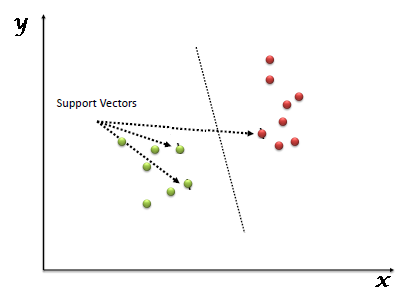
Here, maximizing the distances between nearest data point (either class) and hyper-plane will help us to decide the right hyper-plane. This distance is called as Margin.

In the next blog I will be talking about my my week-8 which is totally about Unsupervised learning.

Image source-www.analyticsvidhya.com

Spam Classifier

Spam Classifier is one of the basic project we do implementing Machine Learning. While building the projects there are some key points which we need to keep in mind:-

Collect lots of data(Collect those word which occur frequently in spams)
Take sophisticated features(which gives header in spam emails)
Develop algorithms to process your input in different ways (recognizing misspellings in spam). Collect lots of data(Collect those word which occur frequently in spams)

One of the major thing in Machine Learning, after creating the model, we must know how to analys error:-

Start with a simple algorithm, implement it quickly, and test it with your new training sets.
Plot learning curves to decide if more data, more features, etc. are likely to help.
Manually examine the errors on examples in the cross validation set and spotting the trend in error is also important thing in error analysis.

In the next blog, we will see Support Vector Machine.

Bias vs. Variance

In this section we will learn about bias and variance which is one the factor of contributing error in our prediction.Not only, by using high degree of polynomial, we can reduce the training error but also by understanding about the Bias and variance.So what actually is Bias and variance?

High bias (underfitting): both Jtrain(Θ) and JCV(Θ) will be high. Also, JCV(Θ)≈Jtrain(Θ).

High variance (overfitting): Jtrain(Θ) will be low and JCV(Θ) will be much greater than Jtrain(Θ).

The is summarized in the figure below:

Above figure is already self-explanatory, there is no need to explain it.

The underfitting and overfitting is explained above which can be reduced to an extend by using the Regularisation term in the linear regression formula in which it depends on the value of lambda.

we see that as λ increases, our fit becomes more rigid. On the other hand, as λ approaches 0, we tend to over overfit the data.

In the next article we will learn about curves.

Evaluation Of Our Hypothesis

Machine learning is not all about creating a data model which can predict the answer based on the given training set but also to improve the efficiency of our Model by checking for errors.

There are many ways to check for error, which can be given as:-

Getting more training examples
Trying smaller sets of features
Trying additional features
Trying polynomial features
Increasing or decreasing λ

To make it more efficient process of finding errors, the traing set example can be split up into two set which are known as training set and a test set.

Typically, the training set consists of 70 % of your data and the test set is the remaining 30 %.

The new procedure using these two sets is then:

Learn Θ and minimize Jtrain(Θ) using the training set
Compute the test set error Jtest(Θ)

The test set error

For linear regression: Jtest(Θ)=(1/2mtest)∑(hΘ(x(i)test)−y(i)test)2
For classification ~ Misclassification error (aka 0/1 misclassification error):

err(hΘ(x),y)= 1 if hΘ(x)≥0.5 and y=0 or hΘ(x)<0.5 and y=1 0 otherwise

This gives us a binary 0 or 1 error result based on a misclassification. The average test error for the test set is:

Test Error=1/mtest∑err(hΘ(x(i)test),y(i)test)

This gives us the proportion of the test data that was misclassified.

Neural Network-Autonomous Driving

This blog is not the traditional blog but a video blog in which my mentor explained the use of Neural networks in Autonomous Driving i.e. self driving cars which uses the large application of neural networks and works in the following way which you will be seeing in the below video.

The videos has been directly taken from the course which I am taking in Courses. Thanks to Andrew NG for such a amazing content.

Just have a look at the video:-

Direct link for the video is https://www.youtube.com/watch?v=ntIczNQKfjQ

Cost Function and Backpropagation-Neural Networks

After the understanding of Neural networks, you must be how to calculate the h(theta) for the output node of it. There is a way to calculate it which you might be thinking, Yes it the “Cost Function” only. The same cost function which you are using to calculate the logistic regression but with generalization. With generalization only, you can calculate it.

Before giving the formula, let me define some of the terms which I’ll be using the formula, which is:-

L = total number of layers in the network
s_lsl = number of units (not counting bias unit) in layer l
K = number of output units/classes

The formula can be given as:-

Backpropagation Algorithm

“Backpropagation” is neural-network terminology for minimizing our cost function, just like what we were doing with gradient descent in logistic and linear regression. Our goal is to compute:

minΘJ(Θ)

In backpropagation, we can calculate the derivative part of the gradient descent and the algorithm is given as:-

More about back propagation we will study in the next blog.

Application of Neural Networks

Neural Networks can be applied in the wide variety of problems including all the large algorithm which requires extensive paperwork, can be done in few minutes with the help of neural networks.

They started explaining with the help of small examples like simple AND, OR and XOR gate implementation with neural networks. AND gate implementation can be easily understood by looking at the figure located below:-

Here an additional node is inserted which is known as bias node.This node helps to calculate the truth table. Here, we will be using the formula to calculate truth table value which we used to calculate the logistic regression.

The above graph is used to calculate the value of g(z) we will get after its calculation by using the Neural networks.

Week-4 Neural Network

For the first hour, he was trying to motivate us to encapsulate the knowledge of Neural Network because it has great usage in Machine learning and can be used more efficiently other than logistic regression.

Neural Network

Algorithm that try to mimic the brain.Everything we do with our brain like learning and reproducing it when needed, for that Neural network is used. Our brain consist of millions and millions of neuron which has a definite structure consist of input wires called as “Dendrites” and the long output wire called as “Axon“.

So, in neural network, we are also trying to build a algorithm similar to our neuron present in our our brain.We will be building the same the same network that our brain contains the network of neuron.

Implementation

In neural networks, we use the same logistic function as in classification, 1/{1 + e^{- θ ^Tx}, yet we sometimes call it a sigmoid (logistic) activation function. In this situation, our “theta” parameters are sometimes called “weights”.

In this example, we label these intermediate or “hidden” layer nodes a20⋯a2n and call them “activation units.”

a(j)i=”activation of unit i in layer j“.
Θ(j)=”matrix of weights controlling function mapping from layer j to layer j+1″.

The values for each of the “activation” nodes is obtained as follows:
a(2)1=g(Θ(1)10x0+Θ(1)11x1+Θ(1)12x2+Θ(1)13x3)
a(2)2=g(Θ(1)20x0+Θ(1)21x1+Θ(1)22x2+Θ(1)23x3)a
(2)3=g(Θ(1)30x0+Θ(1)31x1+Θ(1)32x2+Θ(1)33x3)
hΘ(x)=a(3)1=g(Θ(2)10a(2)0+Θ(2)11a(2)1+Θ(2)12a(2)2+Θ(2)13a(2)3)

Application of Neural networks will be discussed in next blog.

Logistic Regression

Logistic Regression is the way to get the solution for Classification problem.

Why logistic regression?

If we use linear regression for classification problem which contain only discrete values, it’ll give wavy curve which is not suitable.Hence, we use Logistic Regression for classification.

Cost function will also be changed in logistic regression, it will look like:- J(θ)=1/m∑Cost(hθ(x(i)),y(i))

Cost(hθ(x),y)=−log(hθ(x)) if y=1

Cost(hθ(x),y)=−log(1−hθ(x)) if y=0

With the help of above formulas, we can also write the simplified cost function and gradient descent also.

Cost Function: J(θ)=−1/m∑m[y(i)log(hθ(x(i)))+(1−y(i))log(1−hθ(x(i)))]

Gradient Descent: Repeat{ \

θj:=θj−α/m∑(hθ(x(i))−y(i))x(i)j

}

“Conjugate gradient”, “BFGS”, and “L-BFGS”are more sophisticated and faster way to get the output but it needs more expertise thengradient descent, you can apply this algorithm only when you are well aware of numerical problems. Until, you can use predefined libraries which are already provided in Octave.

You can design your own function to get the result in an efficient manner.

Classification

As already mention in my one of the previous blog, Classification is one of the two types of Machine learning. It is defined as the graph which has been stated in the form based on discrete values obtained from a observation.

We cannot calculate the classification problem simply by linear regression, we have to use some other efficient method which is know as Logistic Regression.

Our new form uses the “Sigmoid Function,” also called the “Logistic Function”:

hθ(x)=g(θTx)
z=θTx
g(z)=1/1+e−z

The following image shows us what the sigmoid function looks like:

How to plot this and make more efficient will see in the next blog.