The Thesis Whisperer

Polynomial Regression & Normal Equation

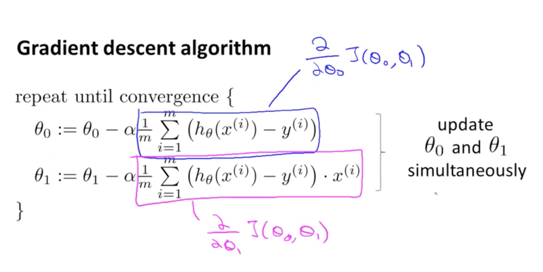
To plot a graph using our dataset is a very crucial part of our prediction. It is not important to fit a straight line, it could also be a polynomial equation. We can have polynomial equations in a graph known as polynomial regression, for example, quadratic function as well as cubic function.

While fitting a particular type of polynomial equation, we have to make sure that our range of different chosen features in our equation must be in the same range.

NORMAL EQUATION

One way of minimizing J is Gradient Descent which takes the approach of the iterative algorithm, another way to reduce the use of this tedious procedure is Normal Equation.

In the “Normal Equation” method, we will minimize J by explicitly taking its derivatives concerning the θj ’s, and setting them to zero. This allows us to find the optimum theta without iteration. The normal equation formula is given below:

Also, there is no use of feature scaling in Normal Equation.

This method can reduce the work but it is also possible that (X^T X)^{-1} is non-invertible, the common cause might be:-

Redundant features, where two features are very closely related (i.e. they are linearly dependent)
Too many features (e.g. m ≤ n).

With this, that’s the end of week-2.

Week 2-Introduction of Octave

It started with the introduction of Octave-Language chosen to implement machine learning.

Octave is a free, open-source application available for many platforms. It has a text interface and an experimental graphical one.
MATLAB is used as software whose license is given by the author to access it free.

After that, they taught me that there could be multiple features like linear Regression with multiple features is known as multivariate linear regression.

hθ(x)=θ0+θ1x1+θ2x2+θ3x3+⋯+θnxn——-this becomes the new hypothesis equation for multiple features.

For multiple variable linear regression, Gradient descent is also very simple to calculate as you can just multiply the single variable formula with x(i)j.

One of the most important concepts is to learn Feature scaling. Feature scaling is to make all the variables range in roughly the same range.

We can speed up gradient descent by having each of our input values in roughly the same range. This is because θ will descend quickly on small ranges and slowly on large ranges, and so will oscillate inefficiently down to the optimum when the variables are very uneven. This can be achieved by:-

-Feature Scaling

-Mean Normalisation.

Mean normalization involves subtracting the average value for an input variable from the values for that input variable resulting in a new average value for the input variable of just zero.

Rest for the next blog…..

My Week 1 Experience Of ML

What I understood about ML is “It is everything in today’s world, without it we cannot live in the age of the Internet”.It taught me what are the new capabilities of the computer.

Two algorithm which I learned is:-
-Supervised learning
In layman’s term, Dataset will be given, from which we have to predict.
-Unsupervised learning
While calculating it, we have no idea what our result should look like.

There are various ways of Model Representation like Line Regression.

The best-suited line in which we can fit into a dataset can be predicted with the help of hypothesis function. Also, we have a way of measuring how well it fits into the data. Now we need to estimate the parameters in the hypothesis function. That’s where gradient descent comes in.

This is the basic Gradient descent algorithm for n=1 since there is a different algo. for n>=1.

Here, In the above figure, we have to use the value of alpha, if it’s too small, gradient descent can be slow otherwise for large values it’ll overshoot the global minimum.

From the further blog, I’ll be posting my day-to-day learnings.

Why this blog?

I have started this blog as my “daily diary”.This personal blog will depict my day-to-day learning which I am pursuing. With the help of my blog, we’ll get to know many things about various ongoing things such as:-

-My C++ and DBMS course on NTPEL.
-My machine learning course by Andrew NG.
-My ongoing project using the concept of ML.

This blog will help me to enhance my learning skills since I am going to write about what I am learning about ML and also my writing skills will enhance.
It will also help me in my revisions when I’ll be in the need of my written stuff which can be easily excessed through my blog.